The Gaussian Is Enough:
Flow-Matching Priors Do Not Help
When Fine-Tuning Large Behavior Models
1Toyota Research Institute 2Woven by Toyota 3Cornell University
*Corresponding author: chen.xu@tri.global
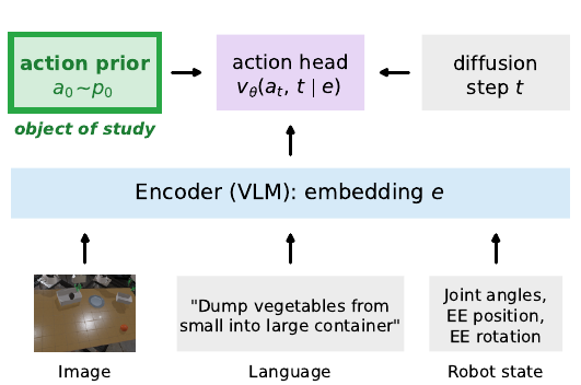
What is the action prior? Left: a flow-matching policy generates an action by transporting a random sample a₀, drawn from a prior distribution p₀ over action chunks, to the target action. The action head is conditioned on the observation embedding e produced by the encoder and on the diffusion step t. By default p₀ is a standard Gaussian; it is the only component we vary. Right: samples from two priors we consider, executed as actions in simulation before flow-matching transport, on the held-out DumpVegetablesIntoContainer task from LBM Eval. The Gaussian 𝒵 produces incoherent, random motion. Apre, the zero-shot actions of the pretrained policy, already makes partial task progress before fine-tuning on task-specific data.
Non-Gaussian action priors that are measurably closer to the target action distribution help when training an imitation learning policy from scratch. We do not observe this benefit when fine-tuning a pretrained Large Behavior Model (LBM). Our diagnostic analyses indicate that the observation encoder, not the action prior, governs fine-tuning performance.
Across over 100K simulated rollouts on three LBM architectures (LBM 1.0, π0.5, and GR00T N1.5) and 40+ tasks, and 1250 hardware rollouts on five bimanual tasks, the standard Gaussian prior performs statistically indistinguishably from, or better than, closer-to-target action priors, with a possible exception at very low fine-tuning data fractions.
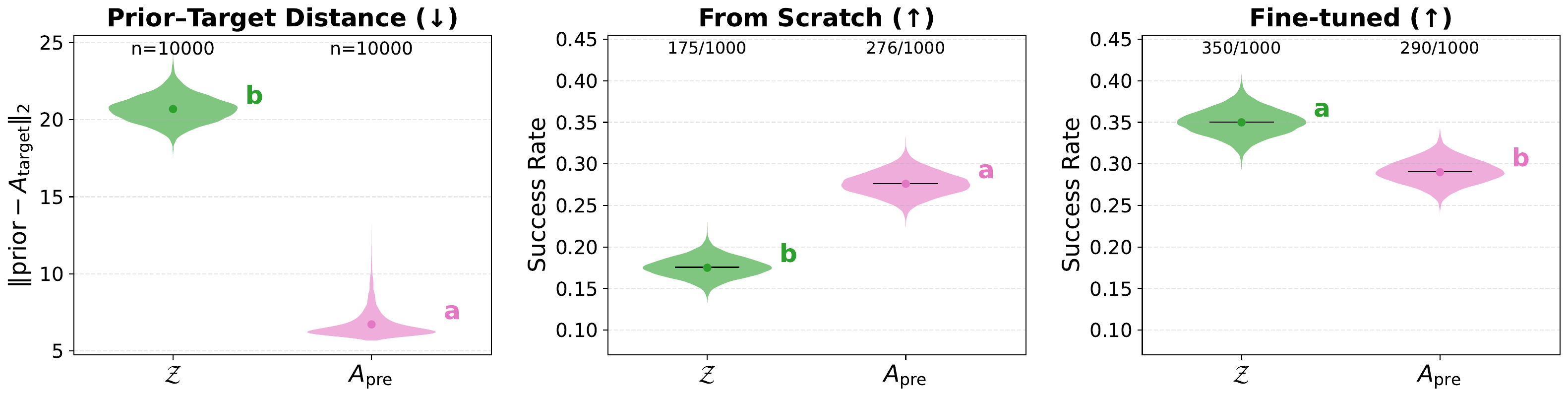
Controlled test in simulation (setting 1 below): five LBM Eval tasks, 1000 rollouts per prior, pairwise comparison of 𝒵 and Apre. Left: ℓ2 distance between prior samples and ground-truth actions; Apre is 3× closer to the target than the Gaussian. Middle: when training from scratch, Apre significantly outperforms the Gaussian. Right: after fine-tuning from the same pretrained LBM 1.0 checkpoint, the Gaussian instead significantly outperforms Apre.
Why a closer prior might help. Flow matching only requires paired samples from the prior and the target, so any distribution can serve as the prior without changing training or inference: the Gaussian is a convention, not a requirement. Recent work exploits this flexibility when training from scratch: BRIDGER (Chen et al., 2024) learns a CVAE action prior, Cocos (Dong et al., 2026) a condition-dependent Gaussian, action-to-action flow matching (Jia et al., 2026) starts from demonstration actions, and EfficientFlow (Chang et al., 2026) adds equivariance guarantees. Replacing the Gaussian with such a closer-to-target prior substantially improves success rates on LIBERO, MetaWorld, and Adroit: if the prior is already near the target, the policy only needs to traverse a short transport distance. Whether this benefit carries over to fine-tuning a pretrained LBM is the question we study.
Experimental Setup
We compare seven action priors: the standard Gaussian, three constructed directly from the pretrained LBM with no auxiliary training, and three baselines from the literature. Within each experiment, only the prior differs; task, data, architecture, optimizer, and training steps are held fixed.
Seven action priors (hover or tap a name):
Clip: samples from this prior executed directly as actions on DumpVegetablesIntoContainer, without a fine-tuned policy or flow-matching transport. Same episode for all seven priors.
Our study is guided by three research questions:
- Q1. Do non-Gaussian priors that are measurably closer to the target improve policy fine-tuning performance?
- Q2. Do informed priors have an advantage across data fractions, particularly in the low-data regime, where the added inductive bias may be most beneficial?
- Q3. Is the effect of prior choice consistent across model architectures, and across simulation and hardware?
Four experimental settings address these questions:
- (1) Controlled test (Q1): a prior constructed to be measurably close to the target, using LBM 1.0 on five LBM Eval tasks in simulation (14,000 rollouts).
- (2) Full-scale fine-tuning in simulation (Q1, Q2): LBM 1.0 on eight LBM Eval tasks unseen during pretraining, at five fine-tuning data fractions (56,000 rollouts).
- (3) Bimanual hardware (Q3): blind A/B testing on five bimanual tasks with two Franka FR3 arms (1250 rollouts).
- (4) Other LBM architectures (Q3): π0.5 and GR00T N1.5 on 34 RoboCasa365 tasks (54,400 rollouts).
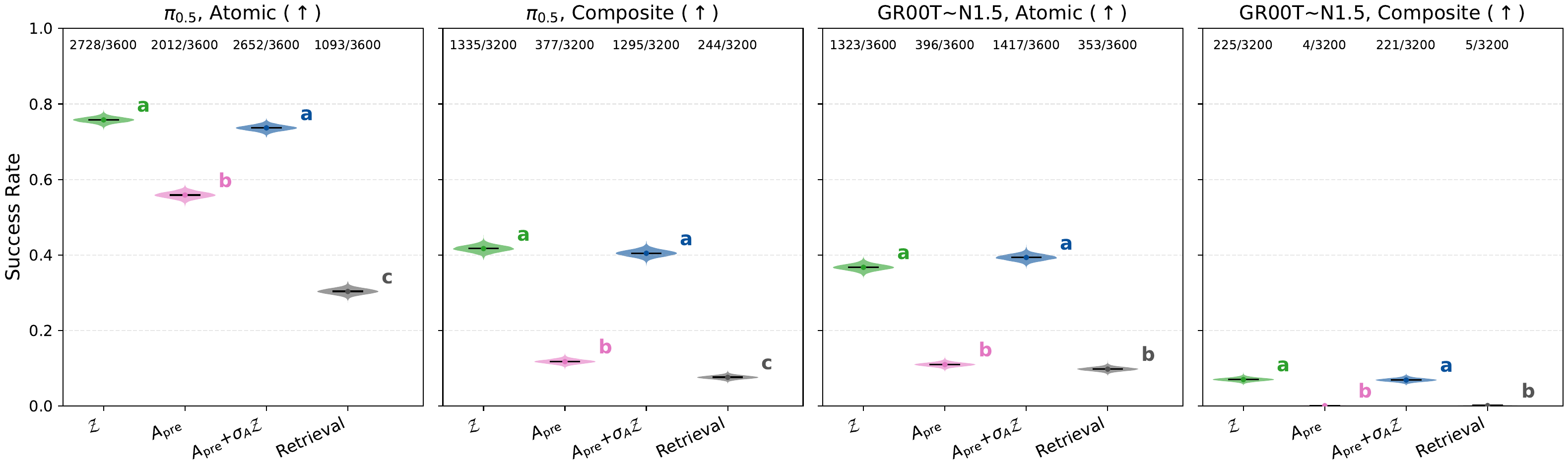
How to read the plots. Success-rate violins show Bayesian posteriors (black tick: posterior mean; dot: empirical mean; counts: successes out of rollouts); violins for continuous metrics show empirical distributions. Each comparison is a hypothesis test (STEP for success rates, Welch's t-test otherwise) at α = 0.05 with Bonferroni correction, summarized as a compact letter display (CLD): priors that share a letter are not statistically separable.
Video speed. Prior-sample clips (at most 20 s) play in real time; fine-tuned policy rollouts are time-compressed to roughly 10 to 12 s, with the factor given in each caption.
Results
(1) Controlled test: a closer-to-target prior helps from scratch, but not after fine-tuning (Q1)
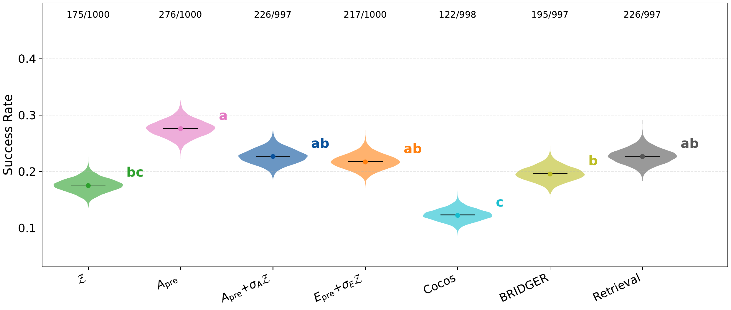
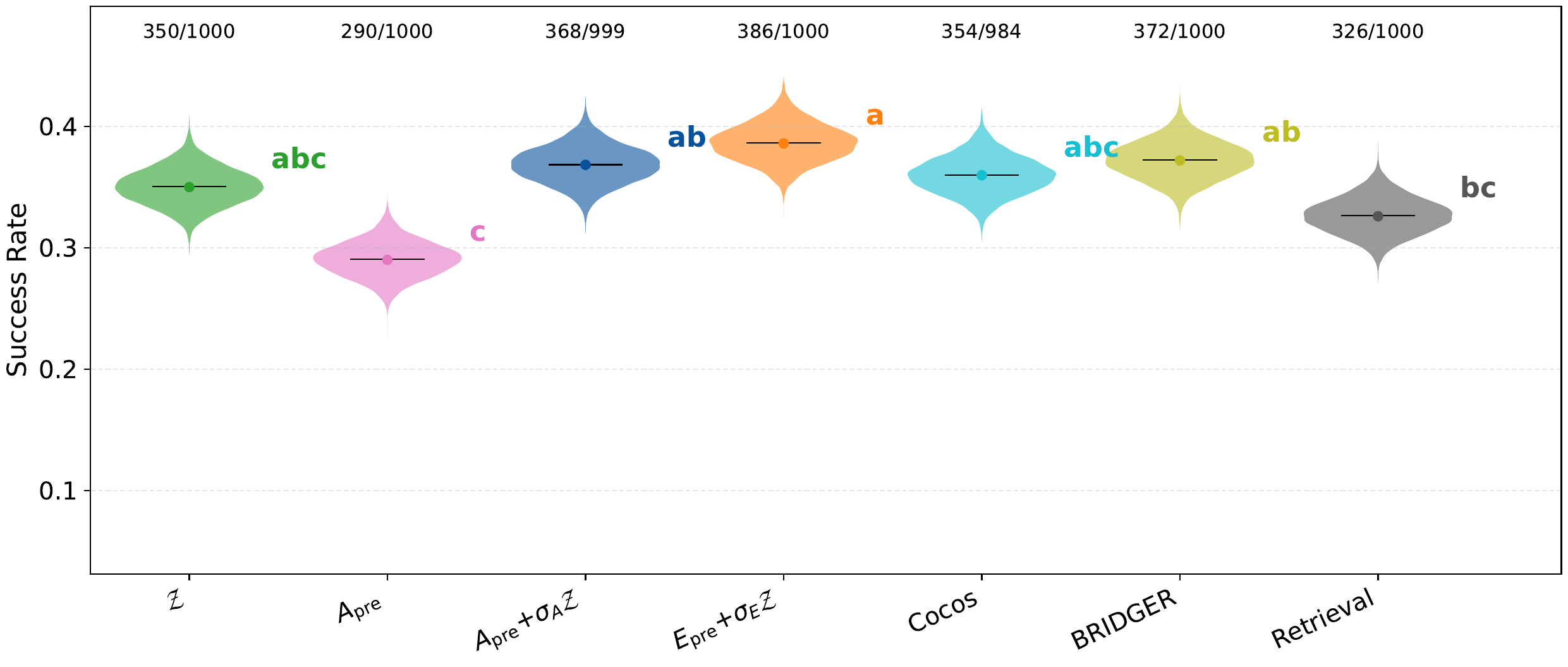
The key challenge in studying non-Gaussian priors for fine-tuning is controlling prior quality: a pretrained LBM has never seen the fine-tuning task, so its zero-shot actions may be out of distribution and form a weak prior. A null result would then be hard to tell apart from a poor-quality prior. We therefore first fine-tune LBM 1.0 with the Gaussian on 50% of the demonstrations, yielding a task-aware checkpoint whose actions are measurably closer to the target, and then fine-tune again from it, varying only the prior. The from-scratch baseline trains the same architecture from random initialization. From scratch, Apre significantly outperforms the Gaussian (roughly 28% vs. 18%). After fine-tuning, Apre becomes the lowest-performing prior, and no prior is statistically separable from the Gaussian in the seven-way comparison.
(2) Full-scale fine-tuning in simulation: priors are statistically tied at every data fraction above 5% (Q1, Q2)
We fine-tune LBM 1.0 on eight LBM Eval tasks unseen during pretraining, using 5% to 100% of the available demonstrations. From 25% upward, all seven priors share CLD group "a". The one exception is 5% (approximately 10 to 20 demonstrations per task), where the embedding-noise prior Epre+σE𝒵 significantly outperforms the Gaussian (25.9% vs. 18.9%); at such low data, the embedding-space perturbation appears to act as an informative inductive bias.
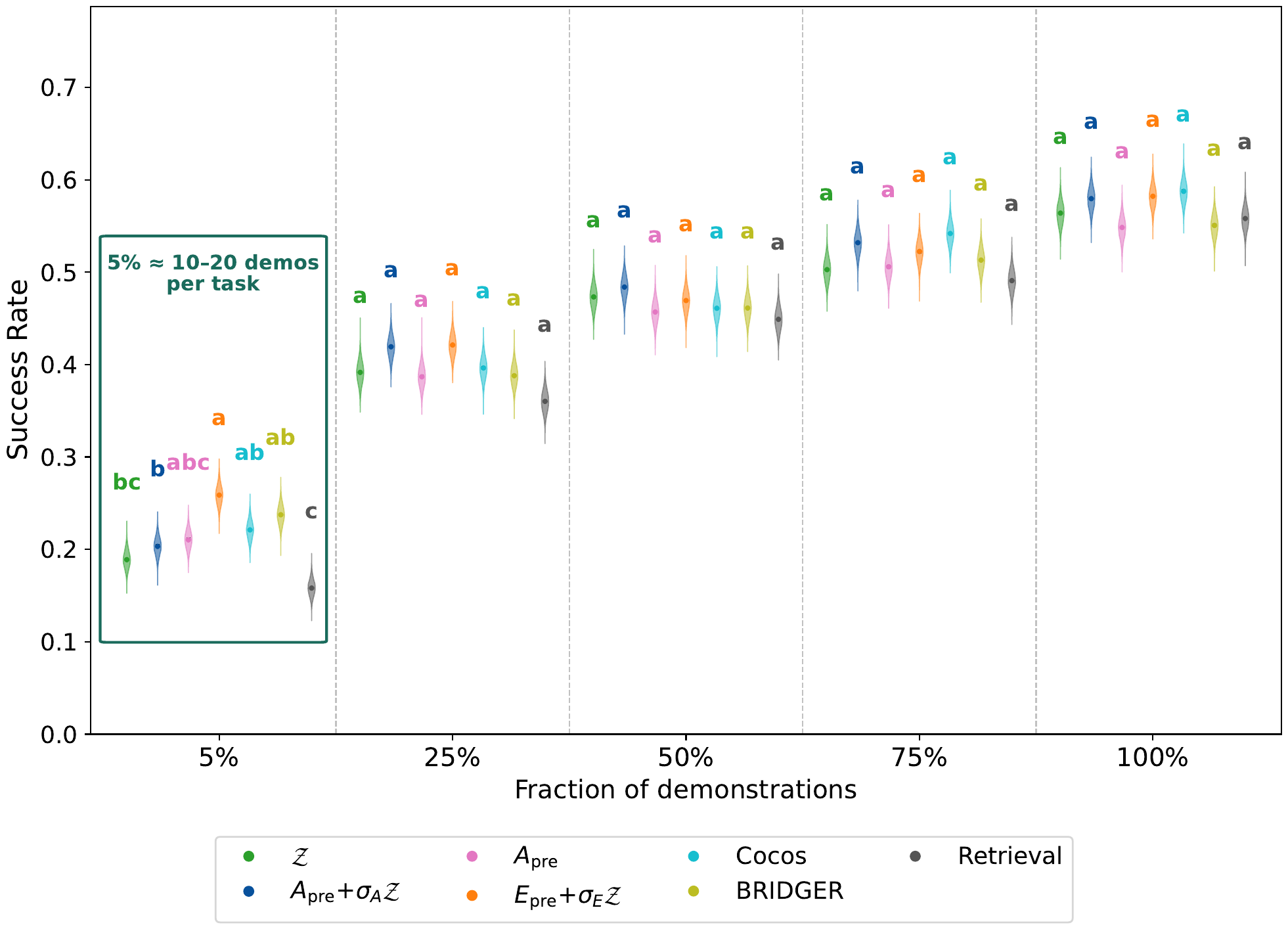
Qualitatively, the seven policies fine-tuned on 100% of the DumpVegetablesIntoContainer demonstrations behave alike when rolled out from an identical initial condition: successes are nearly indistinguishable, while failures show prior-specific failure modes.
To look beyond hand-selected examples, the browser below covers all eight LBM Eval tasks. Each task was evaluated on 200 initial conditions per prior; for visualization we drew 10 of them at random with a fixed seed, so the examples are not chosen by their outcome. Each grid shows the seven fine-tuned policies (100% data) from the same initial condition.
(3) Bimanual hardware: the finding holds on real robots (Q3)
We fine-tune LBM 1.0 on five bimanual tasks with two Franka FR3 arms (FoodBank, ClearKitchenCounter, GatheringIngredientsForCookies, BusBin, BikeRotorInstall) and compare five priors: 𝒵, Epre+σE𝒵, Cocos, BRIDGER, and Retrieval. (A small hardware pilot found our three proposed priors statistically tied, so Epre+σE𝒵 represents them.) In blind A/B testing, following best practices for policy evaluation, all priors are run in randomized order at each initial condition, so the operator does not know which is being tested. Each rollout is scored for binary success and for partial task progress, the fraction of ordered task milestones achieved (e.g., rotor picked up, rotor seated, lockring tightened). Over 50 rollouts per prior per task (1250 total), four of the five priors share a CLD group on both metrics, with partial progress of 71% to 77%. BRIDGER is the sole outlier (about 56%), consistent with its unstable CVAE training.
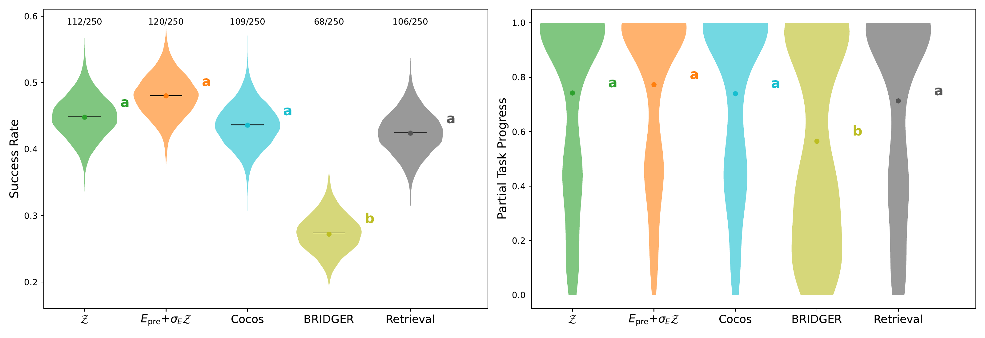
Select a task to see all 250 of its rollouts: each row is one prior and each tile one rollout, individually time-compressed to 10 s and tagged S (success, green) or F (failure, red). Below each grid, a selector lets you view any of the task's 50 initial conditions side by side across the five priors; it opens on one drawn uniformly at random with a fixed seed, so the default example is not chosen by its outcome. For FoodBank and BikeRotorInstall we also show hand-selected initial conditions.
Two hand-selected FoodBank initial conditions show the pattern seen in simulation: at one, all five policies succeed with similar motions; at the other, all five fail in different ways.
BRIDGER never succeeds on BikeRotorInstall, so no initial condition has all five policies succeeding. Below is one where all five fail after comparable progress: each seats the rotor on the hub, then 𝒵 and Retrieval skip the lockring and reach for the tool, while Epre+σE𝒵, Cocos, and BRIDGER place the lockring but drop the tool between the spokes.
(4) Other LBM architectures: the finding holds on π0.5 and GR00T N1.5 (Q3)
We repeat the comparison on the RoboCasa365 benchmark with π0.5 and GR00T N1.5, each fine-tuned on 18 atomic and 16 composite tasks. Neither model exposes a single bottleneck embedding, so the embedding-space priors (Epre+σE𝒵, Cocos, BRIDGER) cannot be ported; we compare the other four. On both models, 𝒵 and Apre+σA𝒵 (pretrained actions plus noise) tie at the top, while Apre and Retrieval are significantly worse, although Apre remains roughly 3× closer to the target in ℓ2. Proximity to the target therefore does not explain the gap. Unlike LBM 1.0, whose pretraining includes data from the same simulator, both models were pretrained mostly on real-world data; this domain gap hurts the two priors that rely solely on a frozen copy of the pretrained model, while we hypothesize that the noise-regularized priors are less affected.
Analyses
How do priors shape the training dynamics and model internals?
In short: different action priors lead to different fine-tuned encoder representations, but these are equally predictive of the target actions. Once the encoder is sufficiently well pretrained, it governs policy performance; the action prior does not.
(1) Fine-tuned encoders are equally predictive of the target actions
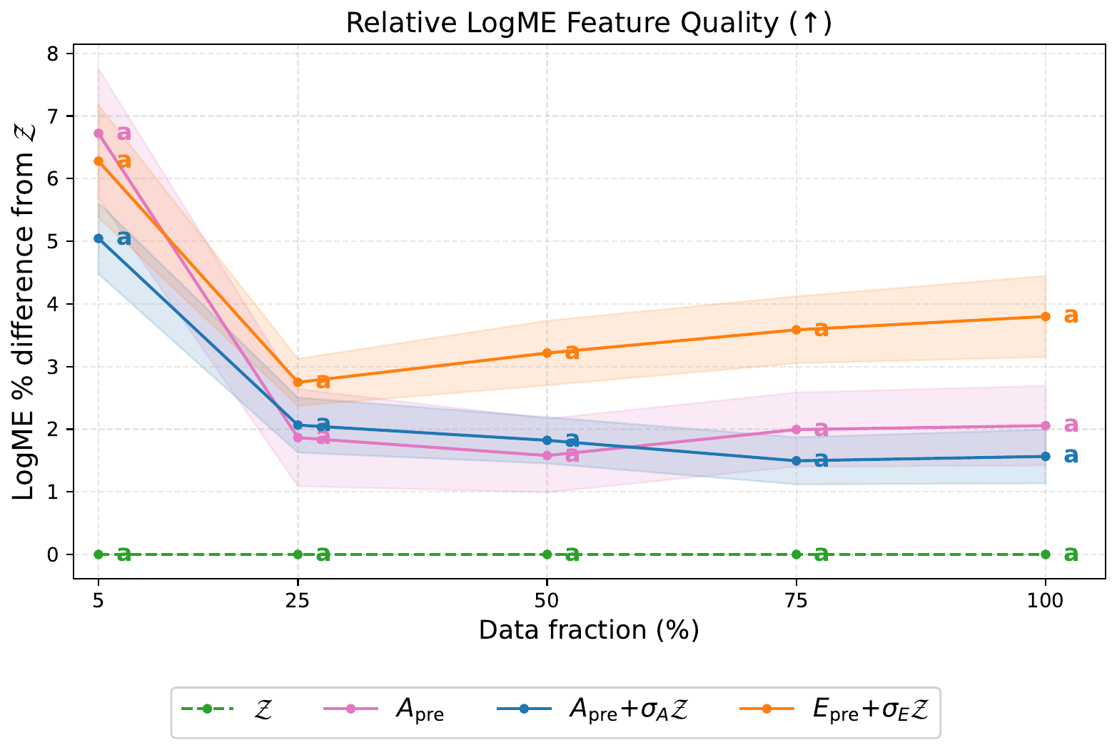
LogME is a training-free measure of feature quality: the log marginal evidence of a Bayesian linear regression from the fine-tuned encoder's embeddings to the ground-truth actions. Scores are statistically inseparable across priors at every data fraction, so the prior leaves no detectable effect on the quality of the encoder's features.
(2) Encoder representations diverge, action predictions do not
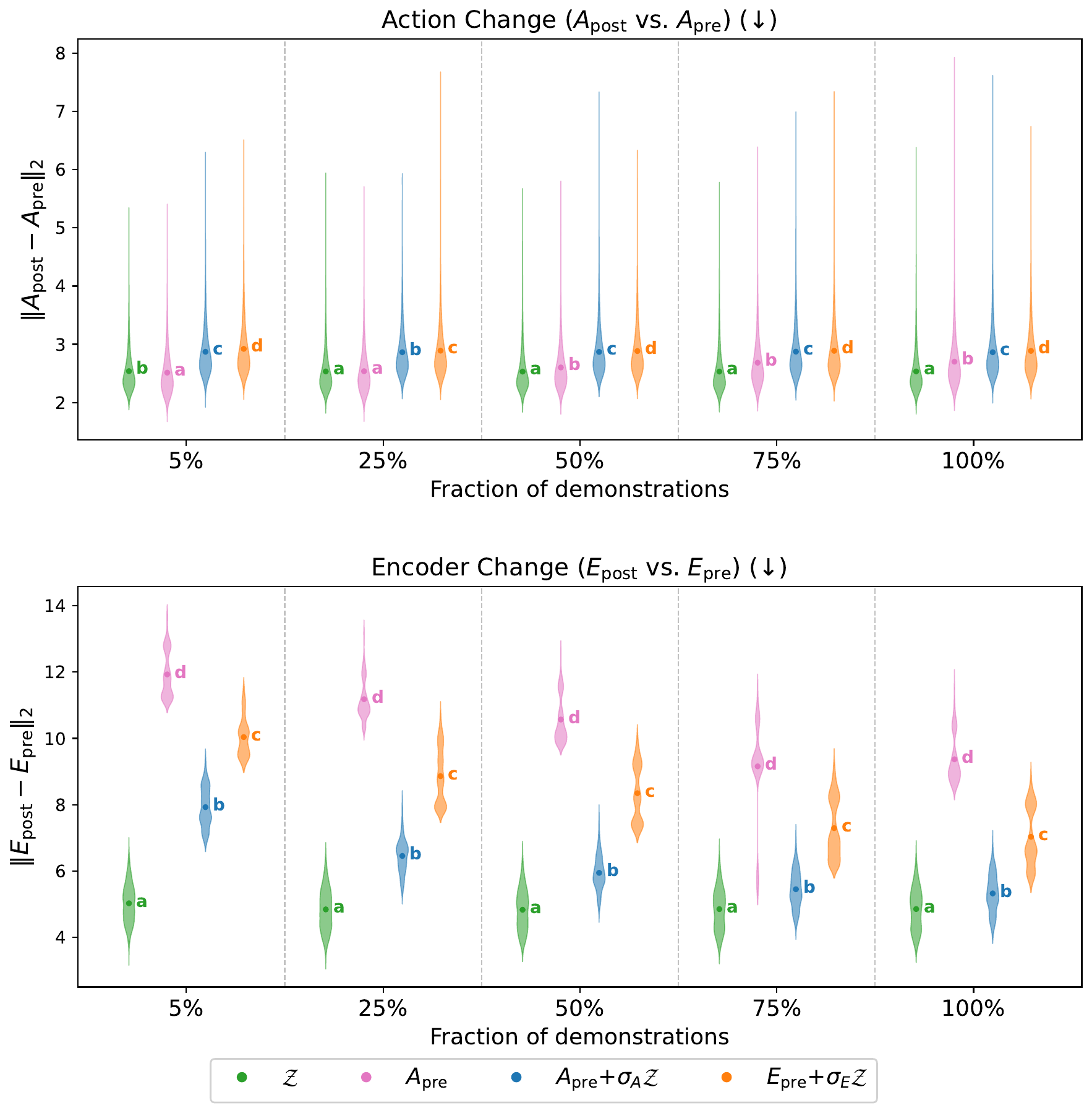
We measure how far fine-tuning moves each model from the pretrained one (per-observation ℓ2 distance). Action predictions change by a comparable amount across priors, but encoder embeddings diverge sharply: the Gaussian moves the encoder least, Apre roughly 2 to 2.5× more. One plausible reason: the Gaussian was also the pretraining prior, so fine-tuning with 𝒵 shifts only the target, whereas Apre shifts both prior and target, and the encoder compensates.
(3) Encoder training matters more than prior choice
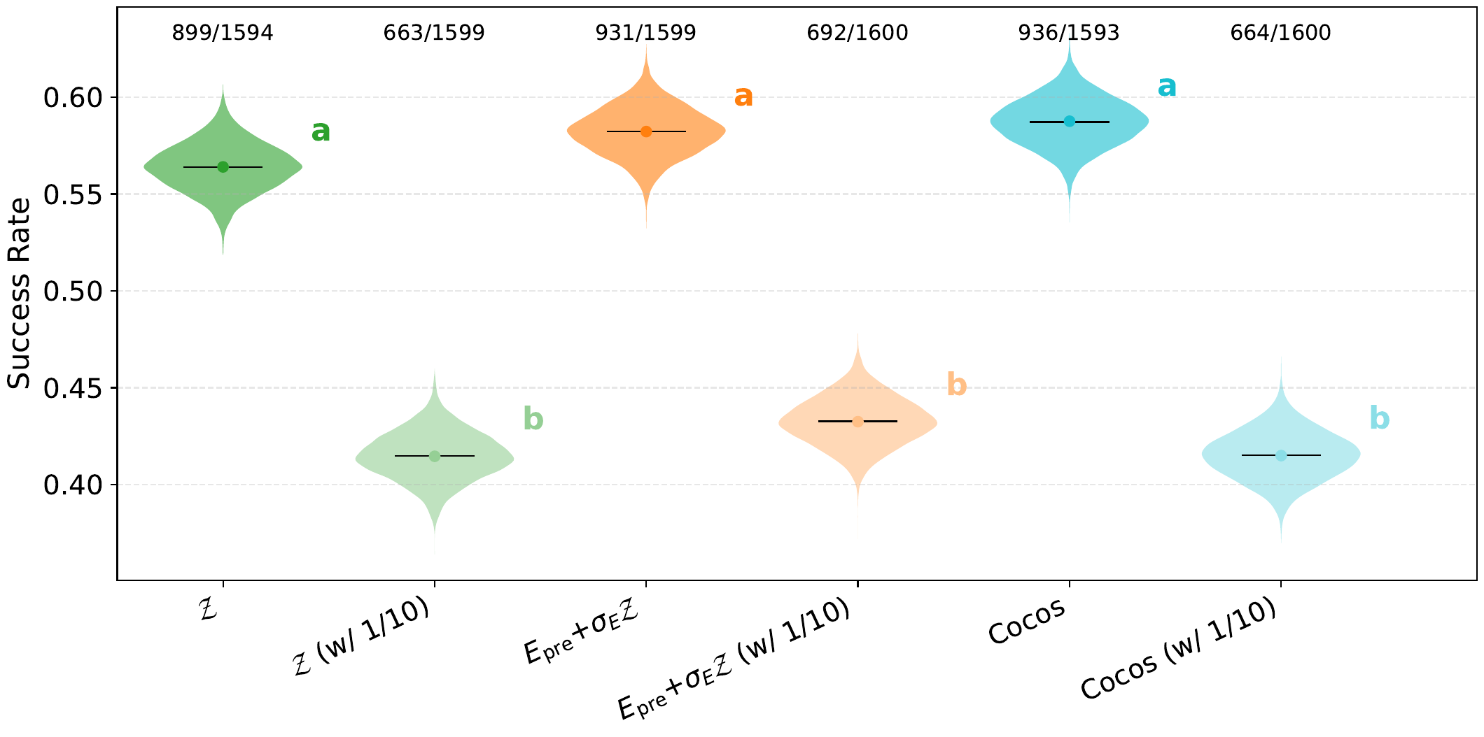
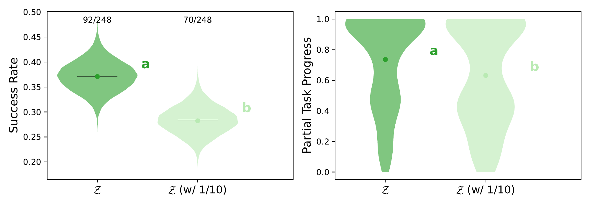
If the encoder dominates, degrading it should hurt far more than changing the prior. We cut the encoder's learning rate to 1/10 of the action head's. In simulation (eight tasks, 100% data; 𝒵, Epre+σE𝒵, Cocos), success drops from 56–59% to 41–43% for every prior, with no measurable prior effect within either learning rate. On hardware (five tasks, Gaussian prior), success drops from 37% to 28%. No change of prior in this study has an effect of comparable magnitude.
Discussion
Implications for practitioners. The standard Gaussian prior is sufficient for fine-tuning LBMs with a flow-matching action head; learned priors add engineering complexity with no measurable benefit. What matters is the quality of the pretrained representations. Without pretraining, learned priors may still be valuable.
Limitations. Our findings cover three LBMs and roughly 10 to 400 fine-tuning demonstrations per task. Much larger or smaller models, other pretraining data, or much larger fine-tuning sets might behave differently, and the encoder-dominance explanation remains a hypothesis at other scales.
Open questions.
- Where is the transition? At 5% data, a learned prior significantly outperformed the Gaussian. Mapping where the prior begins to matter as a function of dataset size, task complexity, and model capacity would tell practitioners when a learned prior is worth its cost.
- Why do different priors yield divergent encoders of equal quality? Loss-landscape geometry, plasticity, and linear mode connectivity are plausible directions.
- Does encoder divergence have downstream consequences? Whether these structurally different encoders differ in robustness to distribution shift, continual-learning stability, or catastrophic forgetting is open.
BibTeX
Preprint: arXiv:2609.27070
@article{xu2026gaussian,
  title={The Gaussian Is Enough: Flow-Matching Priors Do Not Help When Fine-Tuning Large Behavior Models},
  author={Xu, Chen and Shah, Rishi and Kress-Gazit, Hadas and Nishimura, Haruki and Itkina, Masha},
  journal={arXiv preprint arXiv:2609.27070},
  year={2026}
}